Background- Simple Harmonic Oscillator
A simple harmonic oscillator is given by F = -kx where F is force and x is position. Using Newton's 2nd law that gives us:
noting that the term in parentheses on the left is just the velocity (v) and picking k and m such that k/m = 1, we have:
So we want to solve these two. We know of course that the exact solution is x ~ cos(wt) and v ~ -sin(wt) and plotting v vs x will give you a circle, so we can use that knowledge to compare the results. Throughout, I will set my initial values to v(0) = 0 and x(0) = 1 so that the points should lie on a circle with radius = 1 and center = (0, 0) when you plot v vs x.
LabVIEW Example
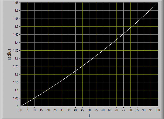
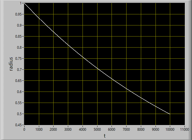
Using the ODE VI in LabVIEW we have a number of different options. We get the following results when we plot v vs x:
x(0) = 1
v(0) = 0
dt = 0.01
final time = 100
algorithm = Euler
x(0) = 1
v(0) = 0
dt = 0.4
final time = 10000
algorithm = Runge-Kutta 4
As you can see from the examples, the Euler algorithm blows up quickly and the 4th order Runge-Kutta trends towards zero. Why?
Explanation
The Euler approximation works by assuming that a point is approximately equal to the previous point plus the slope at that previous point times the difference in x values between the points. That's confusing in words so here it is in math:
Thinking about how that works for a circle...if you take any point on a circle, find the slope (it's the tangent line), and move either clockwise or counter clockwise, you will be closer to zero than the tangent line you found at that x value (sketch it out if it doesn't make sense). Thus, approximating the circle with the tangent line and continuously updating will always give you a slightly larger value. The longer you do this, the more that value blows up. This is exactly what we saw in the LabVIEW plot above that used the Euler method.
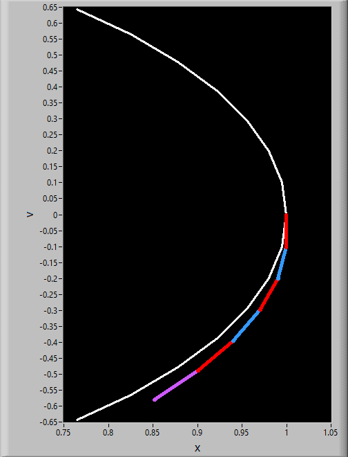
I've zoomed in on the first few iterations of a sample here so you can hopefully see what's going on. Notice that the first tangent (colored) line approximation misses a bit to the right of the circle (white). The next approximation starts with the end of the previous one so it's already high, and it misses high again making the error worse. Each iteration builds on this.
 |
| h = step size; f = differential equation; y = your points |
Thinking about how that works for a circle...if you take any point on a circle, find the slope (it's the tangent line), and move either clockwise or counter clockwise, you will be closer to zero than the tangent line you found at that x value (sketch it out if it doesn't make sense). Thus, approximating the circle with the tangent line and continuously updating will always give you a slightly larger value. The longer you do this, the more that value blows up. This is exactly what we saw in the LabVIEW plot above that used the Euler method.
I've zoomed in on the first few iterations of a sample here so you can hopefully see what's going on. Notice that the first tangent (colored) line approximation misses a bit to the right of the circle (white). The next approximation starts with the end of the previous one so it's already high, and it misses high again making the error worse. Each iteration builds on this.
Putting this into a table, you get the following:
| t | exact x | exact v | real r | approx x | approx v | approx r |
| 0.0 | 1.000 | 0.000 | 1.000 | 1.000 | 0.000 | 1.000 |
| 0.1 | 0.995 | -0.100 | 1.000 | 1.000 | -0.100 | 1.005 |
| 0.2 | 0.980 | -0.199 | 1.000 | 0.990 | -0.200 | 1.010 |
| 0.3 | 0.955 | -0.296 | 1.000 | 0.970 | -0.299 | 1.015 |
| 0.4 | 0.921 | -0.389 | 1.000 | 0.940 | -0.396 | 1.020 |
| 0.5 | 0.878 | -0.479 | 1.000 | 0.901 | -0.490 | 1.025 |
| 0.6 | 0.825 | -0.565 | 1.000 | 0.851 | -0.580 | 1.030 |
Clearly, the tangent line never curves inward as fast as the actual circle does and no matter how small the step size, it will always blow up towards infinity.
The 4th order Runge-Kutta is too long to explain here so I'll just link to the wikipedia article. Suffice it to say though that it experiences a similar problem, except that it trends towards zero instead of infinity. All iterative approximations like this will have errors, and with something like a simple harmonic oscillator or exponential plot that always changes in a consistent way those errors accumulate in the same direction over time. Popular solvers use variants of these, so they're subject to this issue.
It is important to note that some provide ways to set maximum error and they adapt the step size to stay within that, but that's a topic for another post.
Example
Since LabVIEW is less popular than Python, I've provided a simple example in Python instead so that you can experiment with these if you want. To try this out with other differential equations, just change the definition of 'diffEQ' at the top and adjust the parameters as needed (e.g., I needed x and v here...you might just need an x, or maybe you need x, y, and z).
def diffEQ(t, x, v):
 return float(v), float(-x)


import matplotlib.pyplot as plt

#Euler
#Set initial conditions
currentx = 1;
currentv = 0;
currentt = 0;
dt = .001;
xa, va, ta = [], [], []

#Loop over all steps
while currentt <= 400:
 currentt = currentt + dt
 x, v = diffEQ(currentt, currentx, currentv)
 currentv = currentv + dt*v
 currentx = currentx + dt*x
 ta.append(currentt)
 xa.append(currentx)
 va.append(currentv)

#Plot Euler approximations
plt.figure(1)
plt.plot(ta, xa)
plt.ylabel('x')
plt.xlabel('t')
plt.title('Euler')
plt.figure(2)
plt.plot(xa, va)
plt.ylabel('v')
plt.xlabel('x')
plt.title('Euler')

#Runge-Kutta 4
#Set initial conditions
currentx = 1;
currentv = 0;
currentt = 0;
dt = .01;
xa, va, ta = [], [], []

#Loop over all steps
while currentt <= 400:
 k1x, k1v = diffEQ(currentt, currentx, currentv)
 k1x = dt*k1x
 k1v = dt*k1v
 k2x, k2v = diffEQ(currentt + dt/2, currentx + k1x/2, currentv + k1v/2)
 k2x = dt*k2x
 k2v = dt*k2v
 k3x, k3v = diffEQ(currentt + dt/2, currentx + k2x/2, currentv + k2v/2)
 k3x = dt*k3x
 k3v = dt*k3v
 k4x, k4v = diffEQ(currentt + dt, currentx + k3x, currentv + k3v)
 k4x = dt*k4x
 k4v = dt*k4v

 currentx = currentx + (k1x + 2*k2x + 2*k3x + k4x)/6
 currentv = currentv + (k1v + 2*k2v + 2*k3v + k4v)/6
 currentt = currentt + dt

 ta.append(currentt)
 xa.append(currentx)
 va.append(currentv)

#Plot Runge-Kutta 4 approximations
plt.figure(3)
plt.plot(ta, xa)
plt.ylabel('x')
plt.xlabel('t')
plt.title('Runge-Kutta')
plt.figure(4)
plt.plot(xa, va)
plt.ylabel('v')
plt.xlabel('x')
plt.title('Runge-Kutta')
plt.show()
The source code for both the LabVIEW solvers and the python code above is here:
https://github.com/rhamner/ODESolvers


💎 IPRO356💎
ReplyDelete📢 คาสิโนอันดับ 1 เล่นง่ายได้ไว 📢
🔥 มาลุ้นโบนัสก่อนโตได้แล้วที่นี่ที่เดียว
🎮สล็อต บาคาร่า ยิงปลา ไพ่ (ace card) มีจบครบที่เดียว
⚽️ คอฟุตบอล ต้องที่ IPRO356 เท่านั้น เคลียร์บิลรวดเร็วทันใจ จ่ายเลยทันที
💎 สมัครสมาชิก ฟรี ไม่มีค่าบริการ
📱รองรับระบบมือถือทุกรุ่นทั้ง android และ ios
⚖️ ฝาก-ถอน ไม่มีขั้นต่ำ ไม่ต้องทำเทิร์นเลยนะคะ
💸 มีสูตรแจกให้ฟรีพร้อมกลุ่มนำเล่น